
Introduction: People told me that stepwise regression (forward selection / backward / bidirectional elimination) is false, and that LASSO / RIDGE / combination of the two is the best automatic methods. But I dont understand why?
Answer:
Auto-insurance pricing is one of the most sophisticated task within pricing of all insurance products. When there are less than 100 variables to be tested in the model, checking one by one, and building the model step by step remains a good approach. But in the Big Data context, there can be much more variables in the data base, thus we need some kind of automatic feature selection method. Stepwise regression is widely used within regression practionners, yet it violates every principal of statistic, for example:
- It yields R-squared values that are badly biased to be high.
- The F and chi-squared tests quoted next to each variable on the printout do not have the claimed distribution.
- The method yields confidence intervals for effects and predicted values that are falsely narrow; see Altman and Andersen (1989).
- It yields p-values that do not have the proper meaning, and the proper correction for them is a difficult problem.
- It gives biased regression coefficients that need shrinkage (the coefficients for remaining variables are too large; see Tibshirani [1996]).
- It has severe problems in the presence of collinearity.
- It is based on methods (e.g., F tests for nested models) that were intended to be used to test prespecified hypotheses.
- Increasing the sample size does not help very much; see Derksen and Keselman (1992).
- It allows us to not think about the problem.
- It uses a lot of paper.
source: Frank Harell, for more detailled mathematical proofs, please refer to his book.
In my experience, stepwise regression tends to favor very granular predictors over less granular ones, which results in:
- Overfitting.
- Significant loss of information (or Underfitting).
Meanwhile, shrinkage methods is proved to be much more efficient and become one of the state-of-the-art automatic feature selection methods in modern regression. In this post, we will explore at which points shrinkage methods are good, and why.
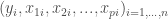
In order to give everyone the same starting point, we need first to understand how a simple GLM / GAM model is built. For simplicity we take an example of linear regression here:

Where 


Suppose that we observe 

In pratice, 

Let 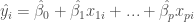


or:

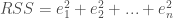
The most common method is Least Square Regression in which we find the value of parameters minimizing the RSS. The solution is:

Fundamentally, 
Why?
It can be proved mathematically that the expected test error (MSE), for a given value of 
![E [y_0 - \hat{y_0}]^2 = Var(\hat{y_0}) + [Bias(y_0)]^2 + Var(\epsilon)](https://s0.wp.com/latex.php?latex=E+%5By_0+-+%5Chat%7By_0%7D%5D%5E2+%3D+Var%28%5Chat%7By_0%7D%29+%2B+%5BBias%28y_0%29%5D%5E2+%2B+Var%28%5Cepsilon%29&bg=ffffff&fg=404040%3B&s=0&c=20201002)
The expected error when applying the constructed model to the new blind data set is the sum of:
- Bias level of the estimates
- Variance of them
- Irreducable error

Above equation tells us that, in order to build a good model performing well on the testing set, we need low variance and low bias.The traditional BLUE (i.e $latex [Bias(y_0)]^2 = 0 $ and $latex Var(\hat{y_0})$ is smallest amongs all the unbiased estimator) is not necessary the best estimator.This method can give us estimators with zero bias, but variance relatively high.
One perfect example of auto insurance pricing relates to the model in which age of the insurer and licence age are included in the model. Or in the Big Data context, external data are included, these variables are associated with regional information and are highly correlated. If we regress frequency / average cost as a log function of insured’s age and insured’s licence age, we will find out that the matrix 

The bias-variance trade – off is well known in modern statistic, there are situations that a little bias can resultto large variance reduction. This is exactly the idea behind LASSO/ RIDGE regression. In order to control the level of 


which is the sum of RSS, plus a component equal to sum of squared parameters, where 

This equation tells us that even in the case of multicollinearity, the matrix that needs to be invert no longer have the determinant close to 0, than the solution doesn’t lead to undesirable variance in estimated parameters. Instead of minimizing bias to 0, and choose between all the unbiased estimator the one with lowest variance, we are minimizing the sum of bias and variance at the same time by playing over different values of
The graph below from @gung at StackExchange helps us to visualize better the bias-variance tradeoff in a clear way:
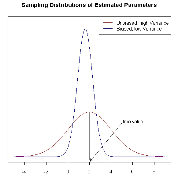
inspired by the discussion on StackExchange: http://stats.stackexchange.com/questions/20295/what-problem-do-shrinkage-methods-solve
DO Xuan Quang
